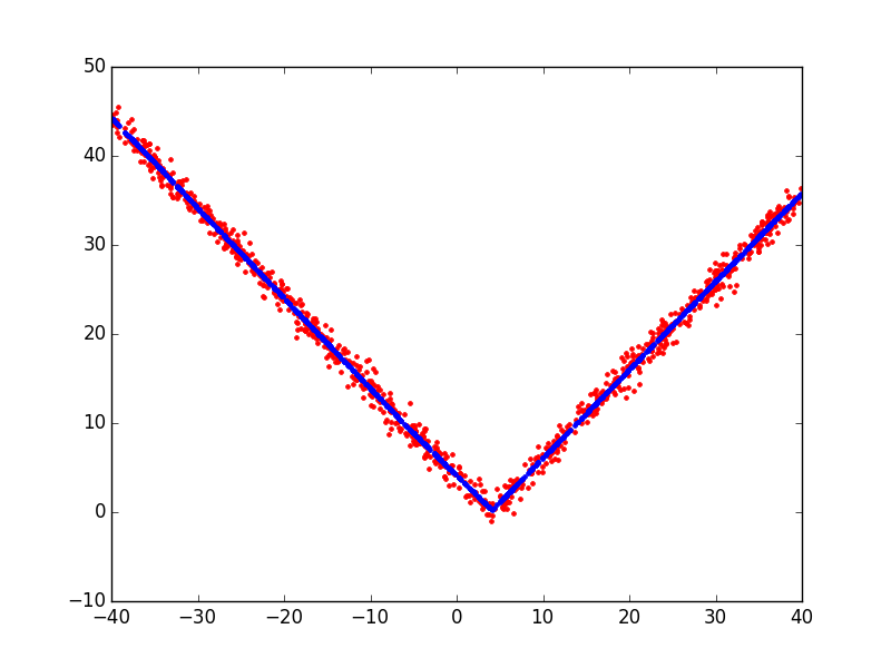
Plotting the absolute value function
A simple example plotting a fit of the absolute value function.
Script output:
Forward Pass
--------------------------------------------------------------------
iter  parent  var  knot  mse         terms  gcv      rsq    grsq
--------------------------------------------------------------------
0     -       -    -     135.278633  1      135.550  0.000  -0.000
1     0       6    441   0.936859    3      0.954    0.993  0.993
2     0       6    569   0.920706    5      0.953    0.993  0.993
--------------------------------------------------------------------
Stopping Condition 2: Improvement below threshold

Pruning Pass
-------------------------------------------------
iter  bf  terms  mse     gcv      rsq    grsq
-------------------------------------------------
0     -   5      0.92    0.953    0.993  0.993
1     3   4      0.92    0.945    0.993  0.993
2     4   3      0.94    0.954    0.993  0.993
3     1   2      84.09   84.932   0.378  0.373
4     2   1      135.28  135.550  0.000  -0.000
-------------------------------------------------
Selected iteration: 1

Earth Model
-------------------------------------
Basis Function  Pruned  Coefficient
-------------------------------------
(Intercept)     No      0.242151
h(x6-4.071)     No      0.991805
h(4.071-x6)     No      0.949437
h(x6+5.756)     Yes     None
h(-5.756-x6)    No      0.0642164
-------------------------------------
MSE: 0.9207, GCV: 0.9451, RSQ: 0.9932, GRSQ: 0.9930
Python source code: plot_v_function.py
import numpy
import matplotlib.pyplot as plt

from pyearth import Earth

# Create some fake data
numpy.random.seed(2)
m = 1000
n = 10
X = 80 * numpy.random.uniform(size=(m, n)) - 40
y = numpy.abs(X[:, 6] - 4.0) + 1 * numpy.random.normal(size=m)

# Fit an Earth model
model = Earth(max_degree=1)
model.fit(X, y)

# Print the model
print(model.trace())
print(model.summary())

# Plot the model
y_hat = model.predict(X)
plt.figure()
plt.plot(X[:, 6], y, 'r.')
plt.plot(X[:, 6], y_hat, 'b.')
plt.show()
Total running time of the example: 0.10 seconds ( 0 minutes 0.10 seconds)