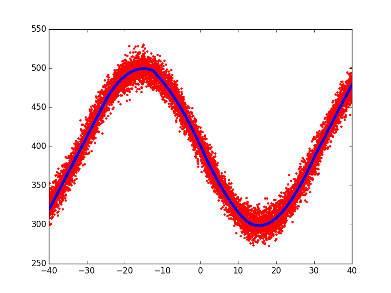
Plotting simple sine function
A simple example plotting a fit of the sine function.
Script output:
Forward Pass
----------------------------------------------------------------------
iter  parent  var  knot  mse          terms  gcv       rsq    grsq
----------------------------------------------------------------------
0     -       -    -     4449.337778  1      4450.228  0.000  -0.000
1     0       6    8011  2989.250294  3      2994.638  0.328  0.327
2     1       6    3811  158.477297   5      159.017   0.964  0.964
3     0       6    6511  129.369292   7      130.019   0.971  0.971
4     3       6    1211  109.489114   9      110.215   0.975  0.975
5     5       6    4711  103.378143   11     104.231   0.977  0.977
6     9       6    3811  101.655699   13     102.659   0.977  0.977
----------------------------------------------------------------------
Stopping Condition 2: Improvement below threshold

Pruning Pass
----------------------------------------------------
iter  bf  terms  mse      gcv       rsq     grsq
----------------------------------------------------
0     -   13     101.66   102.659   0.977   0.977
1     2   12     101.66   102.577   0.977   0.977
2     12  11     101.84   102.676   0.977   0.977
3     3   10     103.10   103.865   0.977   0.977
4     7   9      104.23   104.921   0.977   0.976
5     10  8      104.93   105.543   0.976   0.976
6     11  7      106.56   107.091   0.976   0.976
7     5   6      115.62   116.108   0.974   0.974
8     8   5      138.76   139.236   0.969   0.969
9     4   4      251.66   252.312   0.943   0.943
10    6   3      3026.23  3031.688  0.320   0.319
11    9   2      3872.06  3875.935  0.130   0.129
12    1   1      4449.34  4450.228  -0.000  -0.000
----------------------------------------------------
Selected iteration: 1

Earth Model
----------------------------------------------------------------
Basis Function                             Pruned  Coefficient
----------------------------------------------------------------
(Intercept)                                No      576.111
h(x6+24.5573)                              No      -15.37
h(-24.5573-x6)                             Yes     None
h(x6-9.30493)*h(x6+24.5573)                No      1.88872
h(9.30493-x6)*h(x6+24.5573)                No      0.403057
h(x6+12.5446)                              No      9.10831
h(-12.5446-x6)                             No      -9.33602
h(x6-30.3812)*h(x6-9.30493)*h(x6+24.5573)  No      0.0849127
h(30.3812-x6)*h(x6-9.30493)*h(x6+24.5573)  No      -0.0862001
h(x6-1.85328)*h(x6+12.5446)                No      0.403693
h(1.85328-x6)*h(x6+12.5446)                No      -0.183637
h(x6-9.30493)*h(x6-1.85328)*h(x6+12.5446)  No      -0.0935145
h(9.30493-x6)*h(x6-1.85328)*h(x6+12.5446)  No      -0.0123002
----------------------------------------------------------------
MSE: 101.6557, GCV: 102.5768, RSQ: 0.9772, GRSQ: 0.9770
Python source code: plot_sine_wave.py
import numpy
import matplotlib.pyplot as plt

from pyearth import Earth

# Create some fake data
numpy.random.seed(2)
m = 10000
n = 10
X = 80 * numpy.random.uniform(size=(m, n)) - 40
y = 100 * \
    numpy.abs(numpy.sin((X[:, 6]) / 10) - 4.0) + \
    10 * numpy.random.normal(size=m)

# Fit an Earth model
model = Earth(max_degree=3, minspan_alpha=.5)
model.fit(X, y)

# Print the model
print(model.trace())
print(model.summary())

# Plot the model
y_hat = model.predict(X)
plt.plot(X[:, 6], y, 'r.')
plt.plot(X[:, 6], y_hat, 'b.')
plt.show()
Total running time of the example: 4.88 seconds ( 0 minutes 4.88 seconds)